fMRI Preprocessing & Analysis

Experience the task

You're about to do a short version of the exact task the participant performed inside the fMRI scanner.

You'll see either a real English sentence or a string of random letters. Press F if it's a sentence, J if it's strings — as quickly and accurately as you can.

The task takes about two minutes. Complete it to unlock the brain data.

F — Sentence: "The dog chased the ball across the field"

J — Strings: "FKRMP VTJBQ"

Functional data

The BOLD time series — 229 brain volumes, one every 1.5 s.

Drop .nii.gz here or click

sub-01_…_bold.nii.gz

Required for smoothing & GLM stages.

Structural data

A T1-weighted anatomical scan — high resolution, shows brain structure.

Drop .nii.gz here or click

sub-01_…_T1w.nii.gz

Optional — enables structural viewer.

Motion correction

The problem

Participants move their heads during scanning — even fractions of a millimetre cause neighbouring brain regions to appear to "activate" when they haven't. The scanner collects one full brain volume every 1.5 seconds (the repetition time, TR), giving 229 volumes over 5¾ minutes.

The fix — realignment

fMRIPrep estimated how much the head moved at each TR, saving six parameters: three translations (left-right, front-back, up-down in mm) and three rotations (roll, pitch, yaw in radians). These are plotted below. Change the scrubbing threshold and see how many volumes would be discarded for excessive movement.

Click "Plot motion" to see the head movement trace.

Python code

import pandas as pd
import numpy as np

confounds = pd.read_csv('sub-01_desc-confounds_regressors.tsv', sep='\t')

# Framewise displacement: total head movement between consecutive volumes
cols  = ['X', 'Y', 'Z', 'RotX', 'RotY', 'RotZ']
delta = confounds[cols].diff().fillna(0)
delta[['RotX', 'RotY', 'RotZ']] *= 50  # radians → mm at cortical surface
FD = delta.abs().sum(axis=1)

bad = FD[FD > 0.5]
print(f'{len(bad)} volumes exceed scrubbing threshold')

Slice timing correction

The problem

The scanner doesn't capture all brain slices at the same moment. In a 1.5 s TR, 43 slices are collected one after the other — so the first slice is acquired at t = 0 ms and the last at t ≈ 1,465 ms, almost a full TR later. This means that the "same" volume actually contains brain activity from slightly different time points in different slices. When the GLM later assumes all slices were measured at the same moment, this timing mismatch introduces a small but systematic error in the activation estimates.

The fix — temporal interpolation

Each slice's time series is shifted back to a common reference time using interpolation. The plot below shows when each slice is actually acquired within the TR (left), and how the HRF-convolved signal from an early-acquired slice differs from a late-acquired one before and after correction (right).

Acquisition order

Click "Show slice timing" to visualise the correction.

Python code

from scipy.interpolate import interp1d
import numpy as np
import nibabel as nib

img  = nib.load('sub-01_task-languagelocalizer_desc-preproc_bold.nii.gz')
data = img.get_fdata(dtype=np.float32)
nx, ny, nz, nt = data.shape
tr  = 1.5

# Time at which each slice is acquired within a TR (sequential example)
t_acq = np.arange(nz) * tr / nz   # slice 0 → 0 ms, slice 42 → 1465 ms
t_ref = 0.0                         # reference: align everything to slice 0

# Correct one voxel's time series from the last slice
ts   = data[22, 26, -1, :]            # pick a voxel in the last (latest) slice
t_orig = np.arange(nt) * tr + t_acq[-1]
t_corr = np.arange(nt) * tr + t_ref
f      = interp1d(t_orig, ts, kind='linear', fill_value='extrapolate')
ts_corrected = f(t_corr)

Spatial smoothing

The problem

Individual voxels are noisy — the signal from any single voxel is weak and unreliable. Neighbouring voxels tend to share the same underlying neural activity, so averaging across nearby voxels improves the signal-to-noise ratio.

The fix — Gaussian smoothing

A Gaussian kernel replaces each voxel's value with a weighted average of itself and its neighbours. The kernel width is described by its full-width at half-maximum (FWHM). A wider kernel means more signal but less spatial precision. Each voxel in this dataset is 4.5 mm — try 2 mm, 6 mm, and 20 mm to see the trade-off.

Smoothing kernel (FWHM)

mm — try 2, 6, or 20

Set a kernel size and click "Apply smoothing".

Python code

import nibabel as nib
from nilearn.image import smooth_img

img = nib.load('sub-01_task-languagelocalizer_desc-preproc_bold.nii.gz')
print('Shape:', img.shape)  # (45, 53, 43, 229)  →  x, y, z, time

# FWHM controls the trade-off: larger → more signal, less spatial detail
smoothed_img = smooth_img(img, fwhm=6)  # try 2 or 20 to see the difference

Spatial normalisation

The problem

Every person's brain is a different shape and size, sitting at a different position in the scanner. If we want to compare activation maps across participants, we need all brains in the same co-ordinate system — so that a given (x, y, z) position means the same brain region in every participant.

The fix — registration to MNI152 standard space

Each brain is non-linearly warped to match the MNI152 template (an average of 152 brains). After normalisation, co-ordinate (x, y, z) refers to the same brain region in every participant. This step is performed by fMRIPrep — the file you uploaded is already in MNI space.

Loading images…

Python code

# Normalisation is done by fMRIPrep using ANTs (Advanced Normalisation Tools).
# It computes a nonlinear warp from each person's native brain to MNI152 space.
# The data we received is already normalised.

from nilearn.datasets import load_mni152_template
mni = load_mni152_template()

# Our BOLD data is already in MNI space —
# co-ordinate (x, y, z) now means the same brain region in every participant.
bold_mni = nib.load('sub-01_task-languagelocalizer_desc-preproc_bold.nii.gz')

Building the design matrix

The problem

After preprocessing we have 229 brain volumes — but we can't simply average the "language" volumes and subtract the "string" volumes. The blood-oxygen response is slow, peaking ~5 s after a stimulus and taking ~15 s to return to baseline. We need a model that accounts for this delay before we can ask "which voxels responded more during language than during strings?"

The fix — convolve with the HRF

The haemodynamic response function (HRF) is a mathematical model of the slow blood-flow response. Convolving each condition's on/off timing with the HRF gives the predicted BOLD signal for that condition. These predicted signals form the columns of the design matrix — the input to the GLM. Change the HRF shape or the high-pass filter cutoff and preview how the design matrix changes.

Enter your experimental events

Each row is one trial: when it started (onset), how long it lasted (duration), and which condition it was. The task alternated Language and Strings blocks of 7 s each, separated by 7.5 s rest.

#	Condition	Onset (s)	Duration (s)

Model parameters

HRF model

shape of the blood-flow response

High-pass filter cutoff

seconds — try 32 or 256

Set parameters above, then click "Build design matrix" to see how each condition's timing is modelled.

Python code

from nilearn.glm.first_level import make_first_level_design_matrix
import pandas as pd, numpy as np

events = pd.read_csv('sub-01_task-languagelocalizer_events.tsv', sep='\t')
# Each row: onset (s), duration (s), trial_type ('language' or 'string')

tr         = 1.5
n_vols     = 229
frame_times = np.arange(n_vols) * tr

# Convolve stimulus timing with HRF → predicted BOLD shape per condition
design_matrix = make_first_level_design_matrix(
    frame_times, events,
    hrf_model='spm',      # haemodynamic response function shape
    drift_model='cosine',
    high_pass=1/128       # removes slow scanner drift below this frequency
)

First-level GLM — activation map

Fitting the model

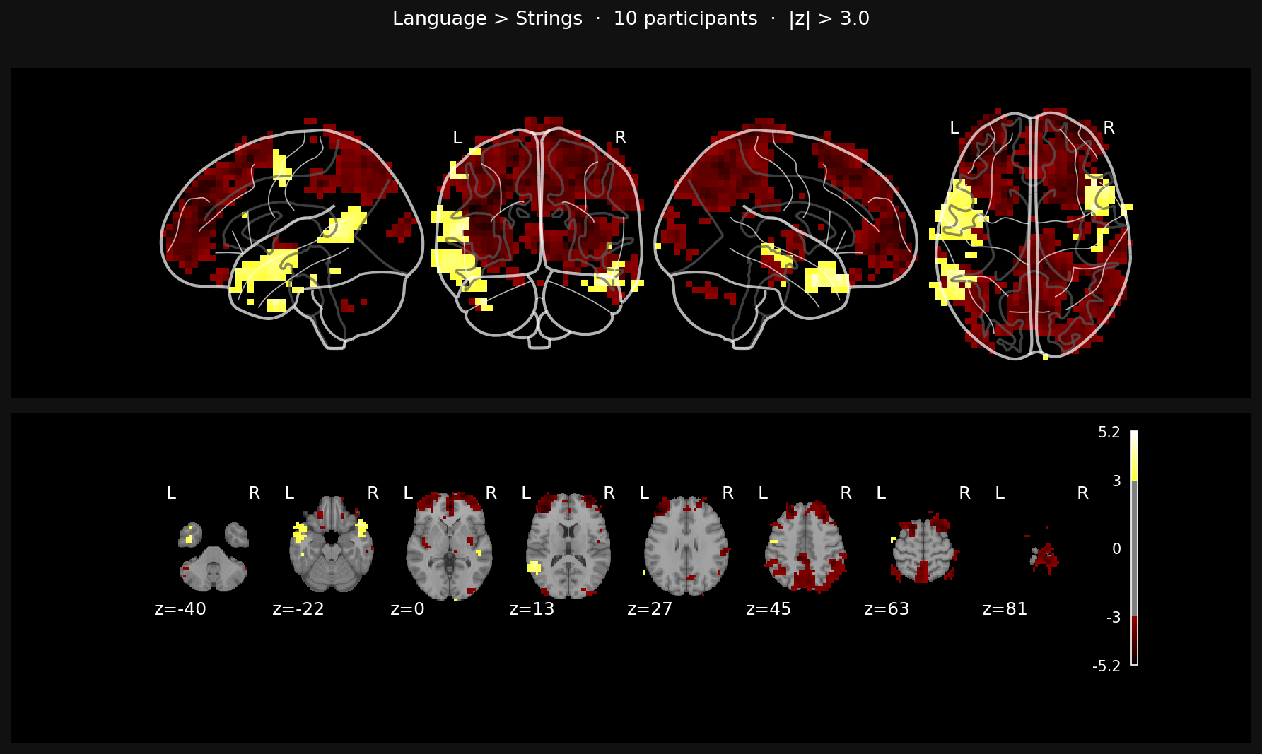
The GLM fits the design matrix to the observed BOLD signal at each voxel independently, estimating how strongly each condition drove that voxel's response. Dividing the estimated effect size by its uncertainty gives a z-score. Voxels with a z-score above the threshold are flagged as "activated". The contrast below lets you ask: which voxels respond more to language, or more to strings?

⬆ Upload your brain scan on the first tab before running the GLM.

Z-score threshold

higher = stricter (try 2 or 5)

Contrast

Language > strings Strings > language

Run the GLM to see the activation map.

Python code

from nilearn.glm.first_level import FirstLevelModel

glm = FirstLevelModel(
    t_r=1.5,
    hrf_model='spm',
    drift_model='cosine',
    high_pass=1/128,
    noise_model='ar1',   # AR(1) autocorrelation correction
)
glm.fit(smoothed_img, events, confounds=confounds)

# z-score: effect size ÷ uncertainty — large = strong activation
z_map = glm.compute_contrast('language-string', output_type='z_score')

fMRI Preprocessing & Analysis

Experience the task

Task complete!

Functional data

Structural data

Brain viewer

Motion correction

The problem

The fix — realignment

Slice timing correction

The problem

The fix — temporal interpolation

Spatial smoothing

The problem

The fix — Gaussian smoothing

Spatial normalisation

The problem

The fix — registration to MNI152 standard space

Building the design matrix

The problem

The fix — convolve with the HRF

First-level GLM — activation map

Fitting the model